This article is actively being developed as of June 18, 2026.
Introduction
Most colors we see come from pigments. A material absorbs some wavelengths of light and sends the rest back to our eyes. Opals are different because their famous play of color is produced by structure. In the broad optics vocabulary, this belongs to structural coloration: color produced by microscopic geometry rather than by pigment.
In precious opal, that structure behaves like a natural photonic crystal. The refractive index changes periodically through the material, and that repeated pattern is small enough to select certain wavelengths of visible light.
This same process shows up across nature. A Morpho butterfly wing, per example can look intensely blue because of nanoscale ridges on its scales. Likewise, a peacock feather shifts color because light is interacting with ordered structures inside each barbule.
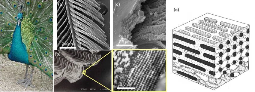
Peacock (Indian peafowl). SEM images of (a) barbules, (b) the cross section and (c) interior of a barbule. (d) TEM image of the cross section of a barbule [112]. (e) Schematic illustration of a 2D photonic crystal in a peacock barbule (reproduced from [111] with permission).
In each case, the material is arranging itself at roughly the scale of visible light, so the color changes when the geometry or viewing angle changes.
The blue comes from tiny ridges and air gaps on the wing scales. Those layers select wavelengths by shape and spacing, much like the silica lattice in opal.
A feather barbule has ordered melanin and keratin structures. As the feather turns, the spacing changes which wavelengths reinforce and which ones fade.
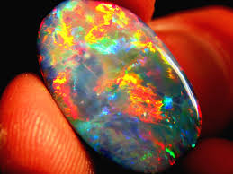
The same structural effect appears across different opal types: dark stones with intense flashes, milky stones with softer color, warm fire opal, and blocky harlequin patterns. Those differences come from body color, domain size, and how clearly each ordered patch is separated from the next one.
 stone
stone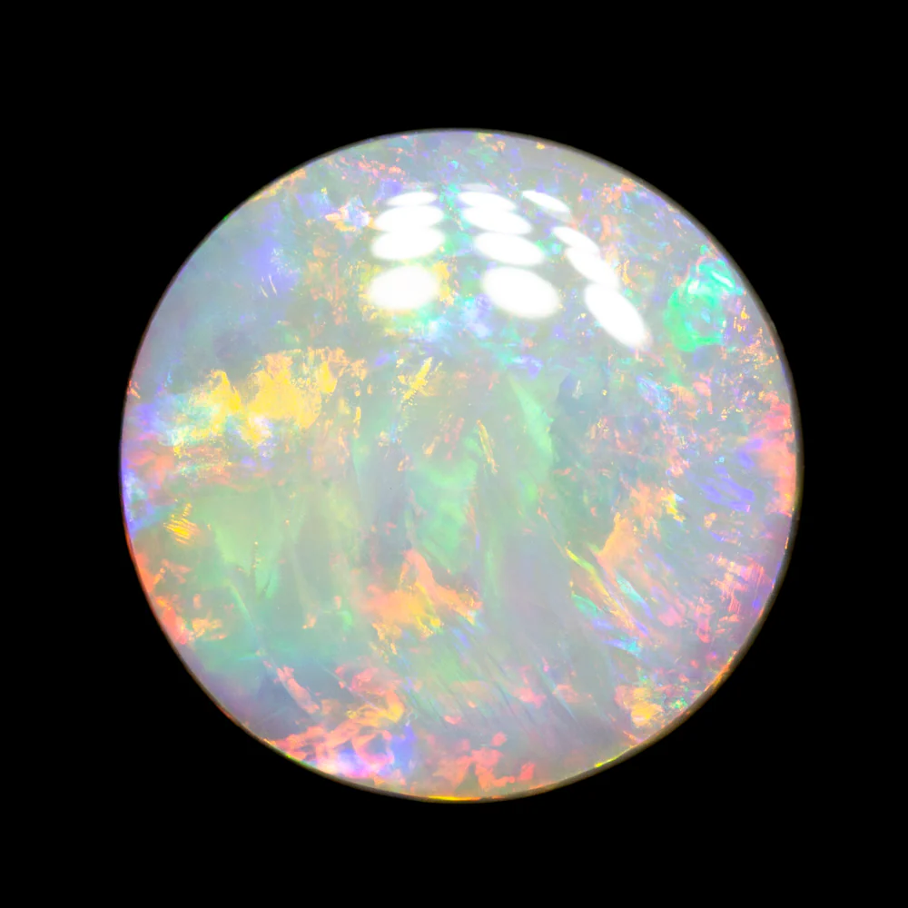 stone
stone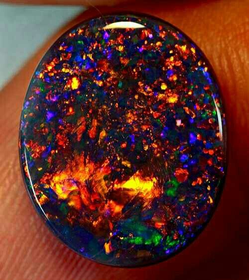 stone
stone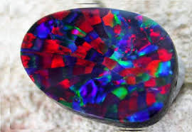 stone
stoneSilica Spheres
An opal begins with silica rich water moving through cracks in rock. Over geological time, the silica settles out into tiny spheres. Those spheres are usually around 150 to 300 nanometers wide, which puts them in the same size range as visible wavelengths of light.
This diameter range matters because it overlaps with visible wavelengths. Much larger spheres would behave more like ordinary grains. Much smaller spheres, on the other hand, would not produce the same strong wavelength selection.
Microscopy
These field emission SEM images from Okudera and Takeda show natural precious opal at the relevant scale: pores left by packed silica spheres, and a fractured wall where distorted spheres show along a crack.
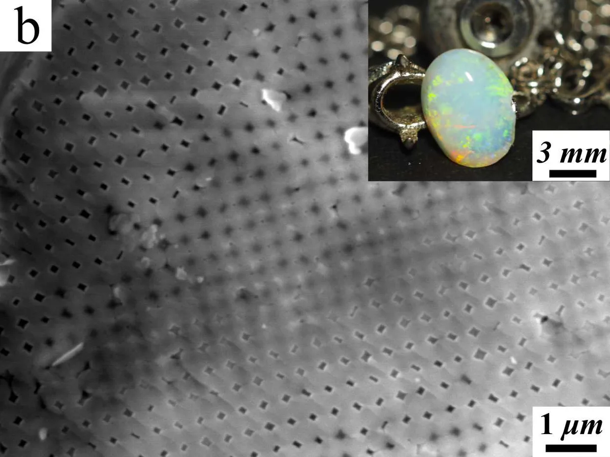
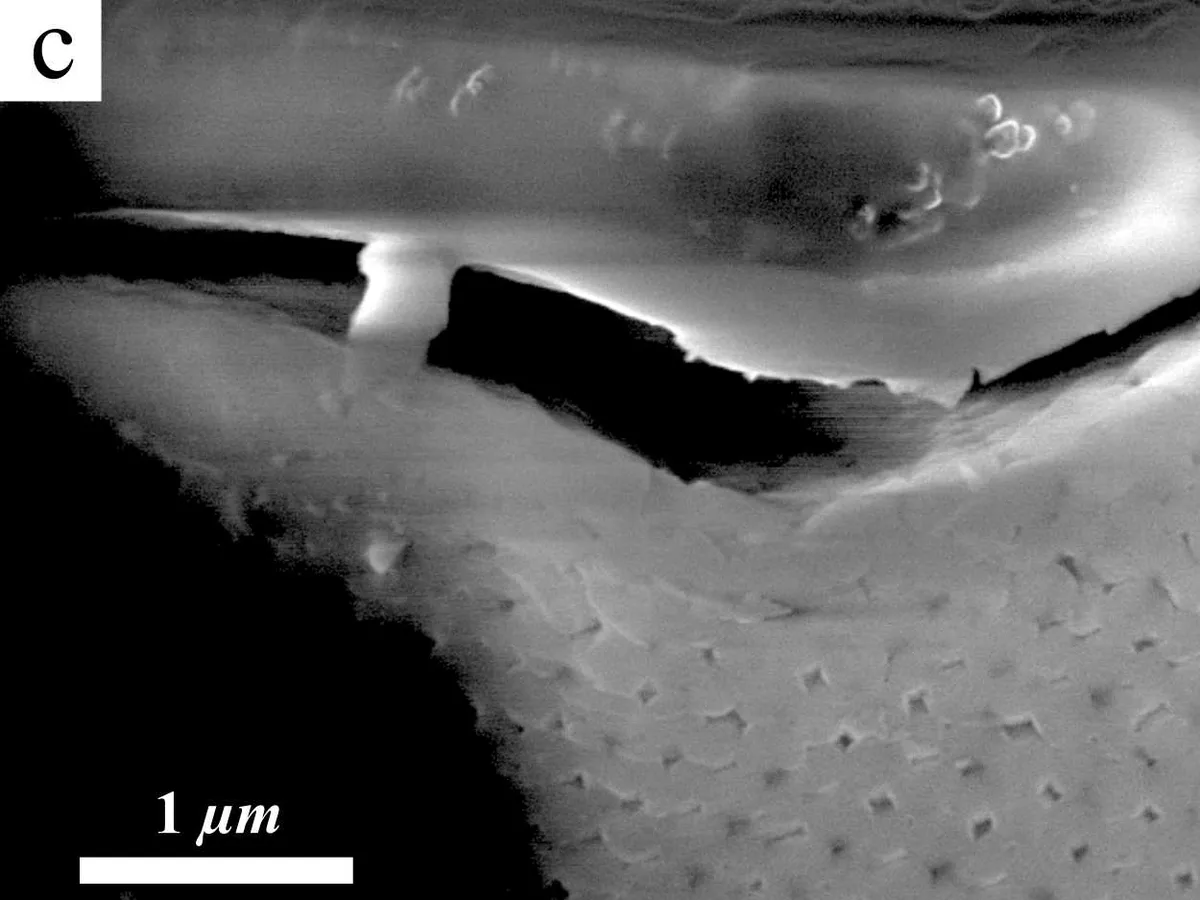
Natural precious opal under field emission SEM. First panel: regular pore pattern in an Australian sedimentary precious opal. Second panel: a fractured wall where packed silica spheres become visible along a crack. Panels adapted from Okudera and Takeda, CC BY 4.0.
Sphere Packing
Close Packing
The silica spheres self assemble into close packed domains, where each sphere sits tightly among its neighbors. In a simplified model, that packing forms a face centered cubic lattice. If the sphere diameter is , the conventional FCC cube has side length:
That relationship connects the sphere diameter to a measurable lattice.
R. Buckminster Fuller’s Synergetics was reference material for the packing sketches.
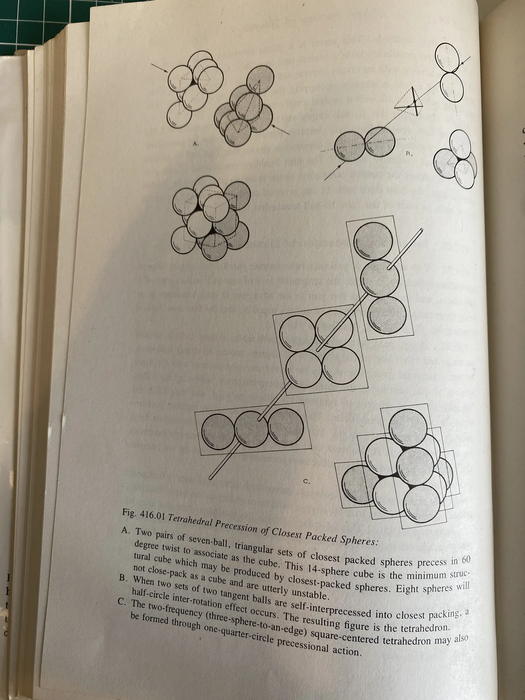
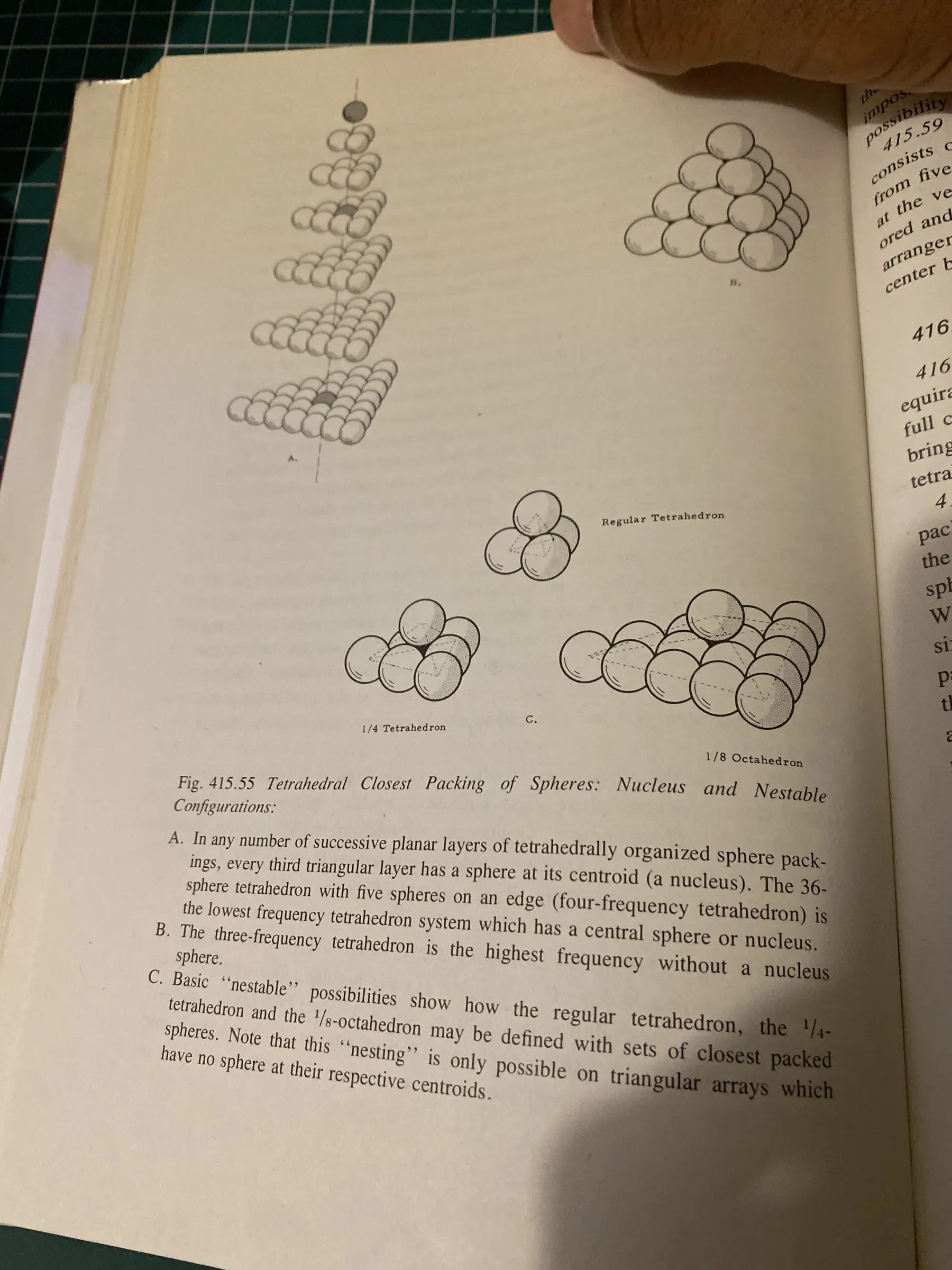
My photos of Fuller’s sphere packing figures in Synergetics. First: Fig. 416.01, “Tetrahedral Precession of Closest Packed Spheres.” Second: Fig. 415.55, “Tetrahedral Closest Packing of Spheres: Nucleus and Nestable Configurations.”
Domains
A real opal contains many ordered domains, each with its own orientation. The slab view shows the layered cross-section. The domain view separates the stone into patches.
Lattice Planes
Miller Indices
Once the spheres are packed together, you can look at them as lattice planes. Different sets of planes cut through the structure at different angles, and each set has its own spacing. For a cubic lattice, a plane family with Miller indices has spacing:
So for the close packed planes in the diagram, the spacing becomes:
That spacing drives the strength of the reflected waves. A smaller spacing pushes the reflection toward shorter wavelengths. A larger spacing pushes it toward longer wavelengths. When an opal has many small crystal domains with different orientations, each patch catches the light a little differently, which is the source of the rich play of color of the stones.
Plane Spacing
Opal play of color recorded as the stone moves relative to the camera. Source: K-Gems Studio.
Bragg Diffraction
The physics behind the flash is Bragg diffraction. Light reflects from many layers inside the opal. At most wavelengths, those reflections cancel each other out, but at the right wavelength and angle, they line up and reinforce each other. The spacing from the previous section follows from the equation below:
Here is the effective refractive index of the opal structure, is the Bragg angle between the lattice plane and the viewing direction inside this simplified slab, and is the diffraction order. The interactive diagram uses , which is the first bright reflection.
Angle Dependence
The same patch, or region of uniform orientation, can move through different colors when the viewing angle changes.
In the diagram, is the acute angle between the reflected ray and the selected lattice plane.
Rendering
Path Tracer
The live render is a smaller version of the path tracer. It uses a low Monte Carlo sample budget, fewer color regions, and a light studio setup with floor shadows so it can run inside the article. I keep the first controls to opal type and body shape, because those are the choices that change the image immediately. The tuning panel is there when you want it: domain size, growth, grid order, preferred tilt, absorption, flash strength, spectral color, and sample budget all pass through to the renderer without taking over the mobile view.
Rendering Iterations
The first versions were simple domain patterns on a sphere. They had the idea of patches, but the patches looked painted on. Then I tried sharper boundaries, random orientations, and stacked layers to create a sense of depth. Each version fixed one problem and made another one obvious.
The small breakthrough occurred when I stopped looking at opals as textures applied to mesh. In an opal, the color inside each patch changes because the viewing angle changes across the surface. A flat color per patch cannot capture that, so the renderer had to follow rays through the structure and let the color come from the geometry.
The explanatory diagram uses Bragg’s law as a direct prediction:
The renderer turns the same idea into a sampling problem. At a domain boundary, a ray with incoming direction tests a small set of reciprocal lattice vectors . Each candidate gives a possible outgoing direction:
where is the grain orientation. A candidate matters when is close to , which means the scattered ray is physically plausible for that wavelength and crystal orientation. I weight those candidates with a narrow diffraction lobe and a simple multi-layer reflection term:
Each pixel accumulates many wavelength samples in CIE XYZ color space:
In plain pseudocode, the renderer is doing this:
for each animation frame:
    if the camera moved:
        clear accumulation

    for each pixel:
        jitter pixel
        lambda = random(380 nm, 780 nm)
        ray = camera ray(pixel)
        xyz = trace(ray, lambda)

        when the ray enters an ordered grain:
            test lattice directions
            sample one diffraction event

        accum[pixel] = running average(xyz)

    display(accum as sRGB)
In JavaScript, the loop is short:
function animate() {
  requestAnimationFrame(animate);
  controls.update();

  if (camMoved(lastCamMat, cam.matrixWorldInverse)) {
    lastCamMat.copy(cam.matrixWorldInverse);
    resetAccum();
  }

  ptMat.uniforms.uCamInvProj.value.copy(cam.projectionMatrixInverse);
  ptMat.uniforms.uCamInvView.value.copy(cam.matrixWorld);
  ptMat.uniforms.uCamPos.value.copy(cam.position);
  ptMat.uniforms.uFrame.value = sampleCount;
  ptMat.uniforms.uSampleCount.value = sampleCount;
  ptMat.uniforms.uAccum.value = accumTarget[0].texture;

  renderer.setRenderTarget(accumTarget[1]);
  renderer.render(fsScene, fsCam);
  [accumTarget[0], accumTarget[1]] = [accumTarget[1], accumTarget[0]];
  sampleCount++;

  displayMat.uniforms.uAccum.value = accumTarget[0].texture;
  renderer.setRenderTarget(null);
  renderer.render(displayScene, fsCam);
}
Inside the fragment shader, each frame contributes one noisy spectral sample. The smoothness of the final fragment color is achieved by averaging the current sample into the previous accumulation buffer:
void main() {
  rngSeed(gl_FragCoord.xy, uFrame);

  vec2 jitter = vec2(rand(), rand()) - 0.5;
  vec2 ndc = (gl_FragCoord.xy + jitter) / uResolution * 2.0 - 1.0;
  vec4 cd = vec4(ndc, -1.0, 1.0);
  vec4 vd = uCamInvProj * cd;
  vd = vec4(vd.xy, -1.0, 0.0);
  vec3 rd = normalize((uCamInvView * vd).xyz);

  float lam = 380.0 + rand() * 400.0;
  vec3 result = trace(uCamPos, rd, lam);
  result *= wl2xyz(lam) * (400.0 / 105.4);

  vec4 prev = texture2D(uAccum, vUv);
  gl_FragColor = vec4(
    (prev.rgb * uSampleCount + result) / (uSampleCount + 1.0),
    1.0
  );
}
Color Space
A glass shell made the edge flare at grazing viewing angles, so I removed it. Some sampling changes made the render cleaner but flattened the color, so I went back to simpler stochastic sampling.
One of the stranger bugs was a persistent pink cast, which turned out to be a color space problem rather than an optics problem. The renderer was mixing values that should have stayed linear until display, so the final image shifted when it was converted back to sRGB.
Citation
If you cite or reuse this project, please cite the article and the renderer:
@misc{sumo_opals_photonic_crystals_2026,
  author = {Sumo, Armand},
  title = {Opals as Photonic Crystals},
  year = {2026},
  month = {May},
  url = {https://armandsumo.com/posts/opals/},
  note = {Interactive article}
}

@software{sumo_opal_path_tracer_2026,
  author = {Sumo, Armand},
  title = {Opal Path Tracer},
  year = {2026},
  url = {https://github.com/a-sumo/opal-pathtracer},
  license = {MIT}
}
References
R. Buckminster Fuller, with E. J. Applewhite, Synergetics; Explorations in the Geometry of Thinking, Macmillan, 1975.
J. V. Sanders, “Colour of Precious Opal”, Nature 204, pages 1151 to 1153, 1964.
S. Kinoshita, S. Yoshioka, and J. Miyazaki, “Physics of Structural Colors”, Reports on Progress in Physics 71, article 076401, 2008.
Anthony G. Smallwood, “35 Years On: A New Look at Synthetic Opal”, Australian Gemmologist 21, pages 438 to 447, 2003.
Hiroki Okudera and Tetsuyoshi Takeda, “Origin of precious opal revisited: Possible quick formation of precious opal”, Research Square preprint, 2021, licensed under CC BY 4.0.
Gemological Institute of America, “Structures Behind the Spectacle: A Review of Optical Effects in Phenomenal Gemstones and Their Underlying Nanotextures”, Gems & Gemology, 2025.
James T. Kajiya, “The Rendering Equation”, SIGGRAPH Computer Graphics 20, pages 143 to 150, 1986.
Matt Pharr, Wenzel Jakob, and Greg Humphreys, Physically Based Rendering: From Theory to Implementation, 4th edition online, 2023.
The public path tracer repository is here: github.com/a-sumo/opal-pathtracer.